Modelling analog circuits in software


#1

Hi everyone,

I'm about to start a journey into modelling analog circuits. The topic has been in my head for some time already and I want to finally get started. What I'm looking for now is some fellows to go through this together. In my experience ping-ponging ideas can greatly improve the experience for everyone and that's why I think it could be great to work on this together.

My goal...

... is to gain a deeper understanding about what matters in analog circuits and how to model some of the relevant behaviour in a DSP. Maybe we create some Axoloti objects for saturation/filters/vcas based on real circuits. But I consider the creation of new objects a side effect. Really, the primary goal, for me, is to learn and tinker.

My background

I'm currently approaching my final thesis in electrical engineering at a university in Germany. I have some background in DSP and signal theory as well as C/C++ programming. Add to that multiple years of experience building synths and synth modules (eurorack, it's a horrible drug). Why am I mentioning this? Because that says a lot about the angle from which I'll approach this topic.

Preferred methodology

To make this fun and interesting for everyone, I'd suggest we try to make things reproducible for everyone. That means we should be clear about what we did and how so we can all follow each others discoveries. Most importantly, I think we should stick to the same circuit until we all decide we want try something else.

My plan...

... is to start simple and slowly move forward. Ideally, I'd like to pick a circuit and build it. Then we can start making a model in the form of an Axoloti object/patch. With the right tools (oscilloscope, ears, circuit simulator, math, ...) we can compare the real thing to our model and slowly work towards a perfect model. If we succeed in one circuit we can pick the next, more complicated one. All of this will require patience and realistic goals.

Here's my roadmap, but this is more of a suggestion than a fixed schedule:

  1. Start with a simple circuit that involves only a minimal number of components, no feedback and preferrably only a single type of semiconductor. (My idea would be a simple diode saturation, but I'm open to anything)
  2. Decide on a realization of this circuit and build a test rig that we can use to measure stuff about this circuit.
  3. Create a specific object/patch to create test signals like certain oscillator shapes, impulses, sweeps, etc. We could use the community library or another github repo for this. That way, we all work with the same test signals and know that we're talking about the same thing.
  4. Setup an Axoloti patch to feed the test signals to both our real circuit and our model. If we use the left audio output to feed our (real) test circuit, we can use the right output for our digital model. That way, we can directly compare the real thing with our model using all kinds of test equipment.
  5. Create a first naive model by using simple math and circuit analysis. No worries about optimization at this point.
  6. From there on it'll be about comparing our model to the real thing by firing all kinds of test signals at it.
  7. If we succeed with our first simple model, I'd suggest we pick the next. I have some ideas about circuits to try.

My worries

All of this may sound like a rigid plan, but to be honest, I'm not even sure if this is the right approach. What do you think? I'm open for any suggestions, so please: Go ahead and let me know what you think about this.

Does all of that sound interesting to you? Let's go!


TheSlowGrowth contributions
#2

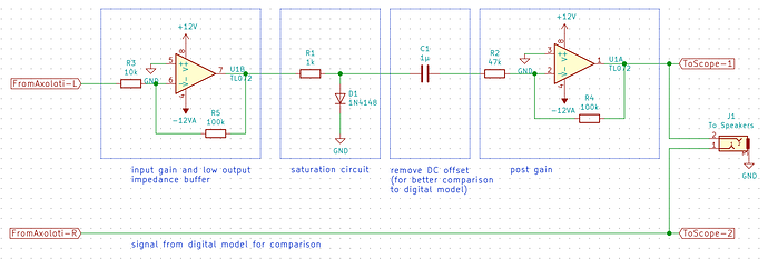
And to get things started, here is a suggestion for a first test circuit. The goal of this could be to find out what's important about a diode distortion. We could later on add a second diode antiparallel to the first to create the typical guitar distortion effect. For now, I think this will give a good starting point.
I guess we will need a high pass filter to compensate for the introduced DC offset with just one diode. Otherwise we may have trouble comparing this to our model.
(warning: I haven't yet built this so I don't know if the gain would be enough).

I'll build this tomorrow and see if it is a good idea, but until then it could serve as a little bait to get you interested :wink:


#3

@TheSlowGrowth, I like your idea, and would love to participate, but I'm not sure I have anything to offer, only basic circuit building experience, and the only DSP knowledge I have is almost nil, except what I have learnt on this forum. But the main reason why I am responding is your choice of first test circuit. "Distortion" From what I have been reading on the great wide web, is that this is a bit of a holy grail search to achieve a true distortion with DSP. Even without extensive knowledge, my attempt at distortion through my "Diode Clipping Simulator" object I posted on the community contributions. But as seams to be the case with most DSP distortion is its lack of random natural feel it has, somehow randomness need to be added to the surface of where the signal is clipped. But I also believe maybe the search for the holy grail needs to end, and in stead of trying to mimic, create something new based on what DSP can achieve that circuitry cannot. The same applies to "Boost" and "Overdrive", as these are part of the family that leads to distortion. This reply is not intended to be negative in any way, as I will watch your progress with great interest and desire to test, but maybe to not follow other DSP distortion attempts to re-create, but more like what is unique about the result. Boost, Overdrive and Distortion is just a topic I am very passionate about but also want to see attempts break down barriers rather then held back by borders.
:grin:


#4

Maybe it is a good idea to study how an electronic modelling software works.
The best exemple is the ubiquitous Spice you may know and use in your studies

That is written in C and open source.
And you can find many tutorials about it.


http://emcs.org/acstrial/newsletters/summer09/HowSpiceWorks.pdf

Personally, i think that many analog cicuits, and especially stompboxes, are particular because buffering is not very high impedance and not linear (NPN common emitter buffers), the different stages are more coupled than chained, this causes many implicit feedback loops... these feedback loops are source of chaotic behaviours that can be the kind of behaviour mentioned by @Gavin ...

One critical issue with distortion in the digital/sampled domain is aliasing.


#5

Okay. So I went ahead and built this small setup.


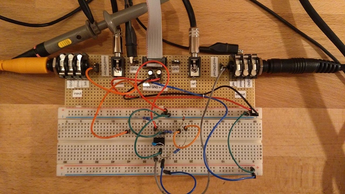
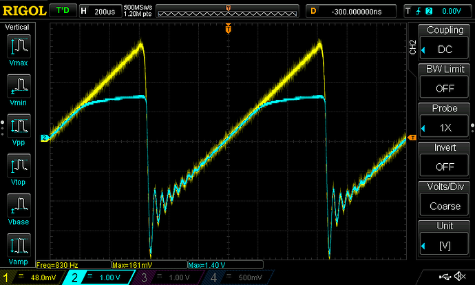
The audio from Axoloti comes in with the orange cable on the left. My soundcard/headphones are connected to the black cable on the right. Power comes from a eurorack case via the ribbon cable. There are some ground hooks for probes and two 3.5mm jacks for connecting a scope (I had the 3.5mm=>BNC cables already and found this less fiddly than standard oscilloscope probes. For audio signal it doesnt make much of a difference anyway)
It is the circuit posted above. Only difference: There is no high pass filter cap and the diode is pointing from ground upwards to the opamp output (due to the inverted signal, this gives me clipping on the positive side of the waveform).

I used this Axoloti patch to send various waveforms to the circuit:
testsignals.axp (28.7 KB)
You can select between Sin/Tri/Saw/Sqr oscillators (both antialiased and not), repeating clicks/pulses, a drum pattern, a synth line and white noise. I'm not sure yet which of these will prove helpful, but it's a start.

I then observed the waveforms on the scope. Here is a zip file with all my measurements: Measurements.zip.axp (1.5 MB - remove the *.axp file extension. I had to rename it to upload)

The measurements I did (+ a few example pics, the rest is in the zip file):
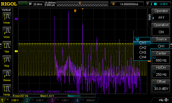
Spectrum of the sine wave I feed into the circuit as well as the spectrum of the distorted waveform with the master volume int he patch set to 32, 45, 55. Here's the distorted version with the level set to 55:

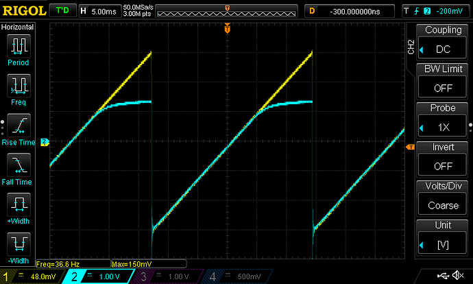
Sin and Saw waveforms with the pitch control set to -38 and +16. Recorded at various levels of dirstorion (32, 40, 45, 50, 55, 64). Here's a saw wave, pitch=-38, level=50:


And the same waveform recorded with the pitch set to +16:

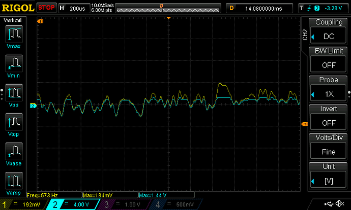
Also I recorded some shots of the Drumbeat. Here's a closeup of the noise portion of a snare hit:

Seems to me like this could be nicely recreated with just waveshaping. I was expecting to see some diode recovery effects on higher frequency signals, but apparently we're not yet high enough to see anything.

Here's a recording of the drumloop. First the source signal, then the distorted signal at levels of 32, 45 and 55 (all normalized so we can hear the effect of the distortion, not just the difference in volume):Drums_src_32_45_55.flac.axp (1.7 MB - again, remove the *.axp file extension)

So, that's all I can do for today, but I'll start creating a simple model later.


#6

Okay, so here's how far I got today.
I wrote down the simple equation that describes the circuit in this picture:
If you sum up all currents flowing out of the node connecting R, Ri and D, you get:

0 = -(10*Uin - Ud)/R + I0*(exp(A*Ud) - 1) + Ud/Ri

where Ud is the voltage between the node and GND, I0 = 50.36µA and A = 7.48336 1/V (which I calculated from two points in the U/I plot in the 1N4148 datasheet).

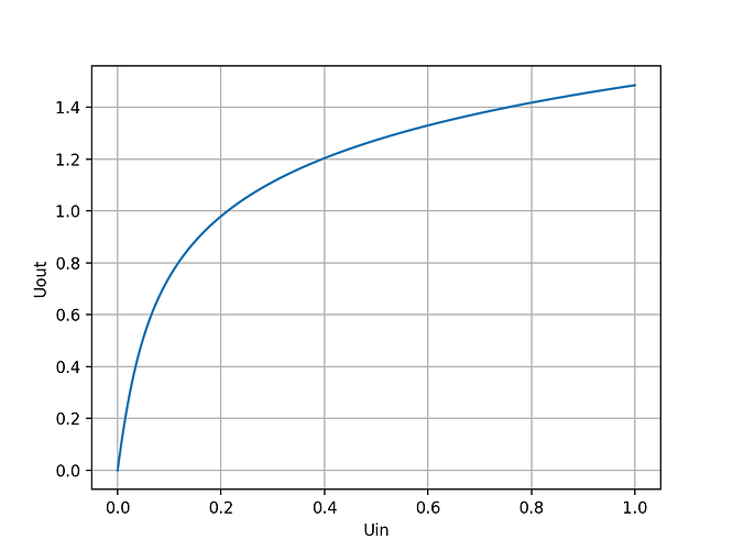
I took the opportunity to finally learn some python (which I wanted to do for a long time). Here's a script that numerically solves that equation for all input voltages between 0-1V and creates the sourcecode for a lookup table to be used in C source code (this could be the start for a actual implementation). Also the script prints a saw and sine waveform together with their distorted signals, which are computed using the lookup table.
Approximation.py.axp (3.2 KB - please remove *.axp file ending)
Please bear with me, it's my first ever python code. Frankly, I was quite surprised how quickly I had put this together.

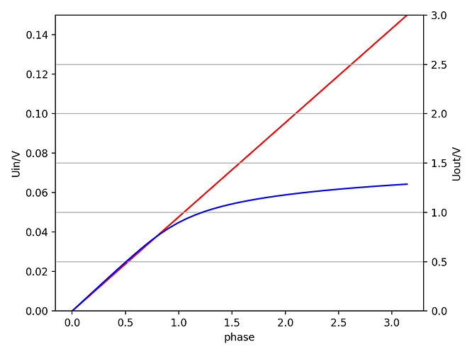
Here's the numerical solution of the above equation:


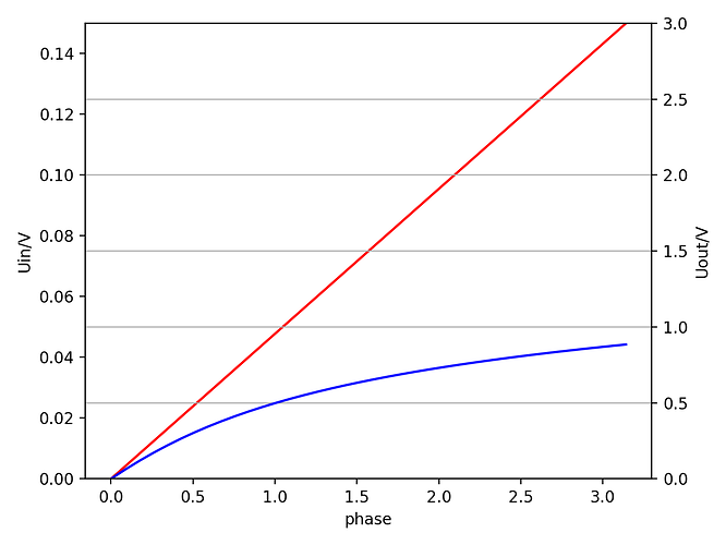
Here's a saw wave and its distorted counterpart, as computed from the equation. This plot is formatted so it can be easily compared to the scope shot from my last post. As you can see its not yet looking anything like the real scope shot, so I guess there's something wrong with my formula so far.
I'm currently trying to figure out why it doesn't show the same image. To me it looks like the diode curve is not quite steep enough, so maybe I picked the wrong values for I0 and A.


#7

Okay, I fixed the issue. Turns out, I had wrong values for I0 and A. I was basically taking wrong readings from the chart in the datasheet.
Now, with the values corrected, this is the new plot:


which looks fairly similar to the real scope shot.

I added the second diode antiparallel to the first to make the distortion circuit complete. In the model, simply only one diode is conductive at a time, which is a good approximation, given that the reverse current in these diodes is so incredibly small.

I then copied the lookup table that was generated by the script into a new axoloti object and added the code that does the interpolation. Right now, it converts to float and does everything super unoptimized. That's why it consumes around 10% CPU (for a simple lookup table read, lol!)
Anyway, here's the object for you to play with:
diodeDist.axo (3.2 KB)

Here is a audio demo comparing the real distorted drums to the model (real first, model second):
real_vs_model.flac.axp (443.2 KB - please remove *.axp file extension)
I can barely hear a difference. To my ears, the model lacks a little bit of top end, but that could just be a subjective thing. I'd say, it's close enough - probably not worth adding any additional stuff to this model, it would only make the computation more CPU intensive.
On the oscilloscope, the real signal and the model look identical now.

Funny, that was way simpler than I had expected.


#8

The optimized (still beta) version can now be found in the community library. TSG/dist/diodeDist.axo
It consumes roughly 6% CPU (still too much if you ask me)

One thing that I found difficult is getting rid of noise introduced by the lookup table. For medium distortion settings and a table size of 256, only the lowest 4 values were actually used! The introduced noise was clearly audible. I tweaked the values a little bit and reduced the maximum available distortion level. Also I increased the size of the table to 1024 values. Now the noise is not audible anymore. Still, it's kind of silly to have a large lookup table, when most of the time you only really use the lowest quarter of it. It would actually be better, if there were more values in the lower ranges and fewer in the higher ranges (were the distortion will mask away any noise that may be introduced by reading from the table).

I'm thinking, a way out of this may be to have multiple, smaller lookup tables for different regions of the curve instead of one single table for the whole curve. I could then dynamically switch between the different tables, depending on where on the curve my input value is. Let's say I originally had a table with 1024 values for the whole input range of -1<28 to 1>>28. That would mean, each value in the table spans over 1<<18 steps of the input.
I could instead have one table of size 512 for the whole range (step size would be 1<<19) and an additional table of size 512 for the range of -1<<22 to 1<<22 (stepsize would be 1<<13). That would be the same memory footprint, but orders of magnitude better resolution in the critical low ranges of the waveform.
The processing would be only marginally more complicated:

if (input < (1<<22))
{
    // read from small table
}
else
{
    // read from big table
}

So that would be an additional shift, subtract and conditional jump operation - that's only very little increase. I'll try this tomorrow and see if the noise can be reduced further.


#9

You could simply have your table be in log scale, although I'm not sure how much CPU that would end up costing.


#10

Yes, but scaling the read index and the fractional would be way too complicated and cost a lot of CPU.

It dawned on me, that lookup tables are not ideal for this application.

  • Not the exact shape of the curve is important (some deviation there wouldn't be problematic) but how smooth the interpolated waveform would be (first order deviation must be continuous)
  • The curve itself is very smooth - a low order polynomial would already be sufficient to approximate the curve well enough.

From there on, its simply a matter of fitting a polynomial into the desired curve. The only important thing is that this polynomial would have to be symmetrical to the origin.
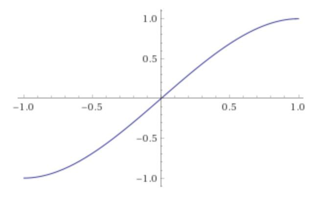
After I realizes that, it dawned on me that this pretty much directly leads to the typical curve found in the dist/soft object in the factory library, which implements this function: y=1.5*x-0.5*x^3 for -1<x<1, y=-1 for x<-1, y=1 for x>1

So - yea - unless I wanted to specifically model the 1N4148 circuit I have here on the breadboard, I could just stop here because I would basically recreate something that exists already.


#11

What if you fit the function with taylor expansions around several points and weigh the single contributions with a table?


#12

That is actually a very nice idea! I wonder how complicated this would get, computation wise. I spent half of this morning trying to fit some polynomials into my curve. I was able to get halfway decent results with 2nd-order polynomials, but only if I split the whole curve into 100 2nd order polynomial sections. The problem with this is that low order polynomials are easy to compute but you need many of them to get decent results. On the other hand you can also (sometimes) get good results with a few high order polynomials - which saves memory but requires many additional multiplications, making it a poor solution for low-powered processors like Axoloti. Right now with my 100 2nd order sections, I don't really save enough memory to justify the increased processing effort.

Coming back to your idea with the weighted taylor sections: I think the same tradeoff applies here. If I use higher order taylor expansions for this, it will be too computationally expensive. If I use lower order taylor expansions, I need more of them, mitigating the benefits alltogether. I might, however get less noise compared to the linear interpolated lookup table.

PS: I also tried to use 5th order polynomials, which are constrained to three points of the curve and the steepness on the points where they touch each other. However, there's still a problem in my equations, I keep getting poorly conditioned equation systems that can't be solved.


#13

could you possibly explain how you derived your equation in more detail?
It’s not something I’ve seen before, or perhaps reference something I could read up on.
Thanks


#14

A few posts back I wrote the equation and also posted an image of the circuit I used to model this.
As you can see, I assumed the operational amplifiers as "perfect amplifiers", so they appear only as abstract amplification blocks, except for the second amplifier, which has a finite input impedance of 47k, which i modeled with resistor Ri.

Now we need the basic equations of each components.
For the resistor, the current/voltage relationship is defined by Ohm's law: R = Ur/Ir. For the 1k resistor: Ur=10*Uin - Ud (Ud is the voltage at the node connecting the diode and the resistor relative to ground.) So that gives: Ir = (10*Uin - Ud)/R. For the 47k resistor that models the imput impedance of the following amplifier stage: Ur = Ud, so that gives: Iri = Ud/Ri
For the Diode, the relationship is Id = I0 * (exp(A*Ud) - 1), where A and I0 are constants that I read from the datasheet. This is the very basic diode equation you will find in every textbook or on every website. Except that I concentrated three values into one constant, A = q/nkT - I don't need to know them all individually.

From there on it's Kirchhoffs law: All currents flowing into a node have to cancel each other out. That leads directly to the equation posted above.


#15

thanks for that, will delve into this with a cup of strong black coffee :slight_smile:


#16

Maybe, you can have a look at Chebychev polynomials approximation. These approximate a function over a segment rather than around a single point.

https://www.embeddedrelated.com/showarticle/152.php


#17

Oh wow, that was a great read. So much valuable information! I'll dive into this a little further. If you have any other links on this topic, don't hold back!

PS: It seems the second link is unfortunately not available anymore.


#18

Here is another like for the numerical recipes chapter:

You can also have a look at Padé approximates, but those need division.


#19

Yesterday I talked to a friend about my efforts in understand analog modelling. He recommended me to this talk. I just watched it and its a wealth of precious information for a beginner like me, and I'm sure everyone here can find some nice inspiration in this - not only for modelling circuits, but also for some general creative patching ideas.

Feedback loops will occur pretty much anywhere, even the circuit I worked on here has feedback, which you can directly see from the form of the equation - it is implicit! To deal with these equations, he suggests to use the Newton Raphson algorithm. I knew about this and the numerical solver in python probably uses this algorithm or something similar. But hadn't thought about using it in real time, because it is very CPU hungry and depending on your exit condition for the algorithm, it can also take different number of iterations to get to a desired result, or not get any result at all - which is something very undesireable in a DSP environment.
One interesting note here is that he suggests to use lookup tables to do the first iterations of the Newton Raphson algorithm, speeding things up immensly. This is something I hadn't yet though of. You don't even need a lot of precision in these tables and you could probably get along just fine with uninterpolated tables - if you use them for the first few iterations of the algorithm, that will get you close to the solution of the implicit equation. You can then refine the result further by doing the last few iterations with the real, CPU hungry equation.


#20

Ok, maybe taylor approximation is not the correct solution. What if instead you do this?

1) the function is antisymmetric, so you don't actually have to fit the whole curve
2) divide the interval in which you want to fit the function in n+1 sections (better if equally spaced).
for each section Si (from x[i] to x[i+1]) you could define a II order polynomial like:

 
a[i] + b[i]*x + c[i]*x^2

This gives you a total of 3*(n+1) coefficients to determine.
3) for the sections S[0], .. , S[n-1] you can define two congruency equations:

a[i]+b[i]*x[i+1] + c[i]*x[i+1]^2 = a[i+1]+b[i+1]*x[i+1] + c[i+1]*x[i+1]^2 (continuity)
b[i] + 2*c[i]*x[i+1] = b[i+1] + 2*c[i+1]*x[i+1] (continuity of the first derivative)

that make up for 2*n constraint equations.
4) You can already say that a[0] = 0 (this makes for another constraint equation)
5) The number of degrees of freedom if 3*(n+1) - (2*n+1) = n+2

Your objective is that to minimize the distance between the sampled function and the polynomial approximation, so that sum(j) (f(x[j])-p(x[j]))^2 ----->0

It's a constrained minimization problem, that you can solve numerically (octave, matlab) by the method of lagrange multipliers.